You can relate to it if you had to grade a long list of students and were not sure about its accuracy. Grading a list of students manually can be time-consuming, especially when you have a large dataset.
With Excel’s VLOOKUP function and its approximate match feature, you can automate this process effortlessly!
In this blog post, I’ll walk you through the steps to generate grades for students based on their marks using a predefined grading system.
Sample Dataset
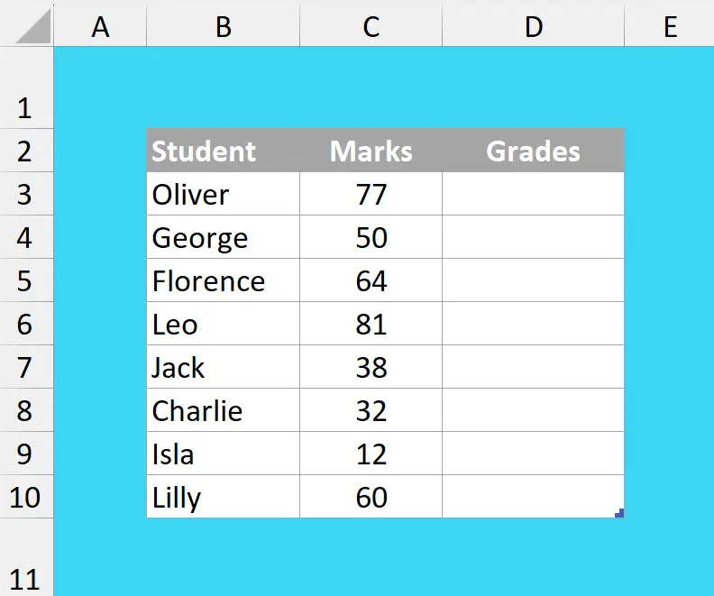
Step 1: Here is a list of students with obtained marks for which you want to do grading.
This dataset doesn't need to be sorted at all for getting the right grades from formula:
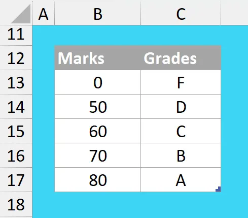
Step 2: There is always a grading scheme that defines the grade ranges. Here is the sample grading we use in this example:
💡The grading scheme must be sorted in ascending order as the VLOOKUP will search for results from top to bottom.
Step 3: In cell D3 write the following VLOOKUP formula for the first student:
=VLOOKUP(C3,B13:C13,2,1)
- C3 is the lookup value
- B13:C13 is the lookup array, which includes two columns, the first column is the search column for lookup value and second column is the result column
- 2 represents the number of column in the table array from which the results are to be calculated
- 1 is to lookup approximate match for the lookup value
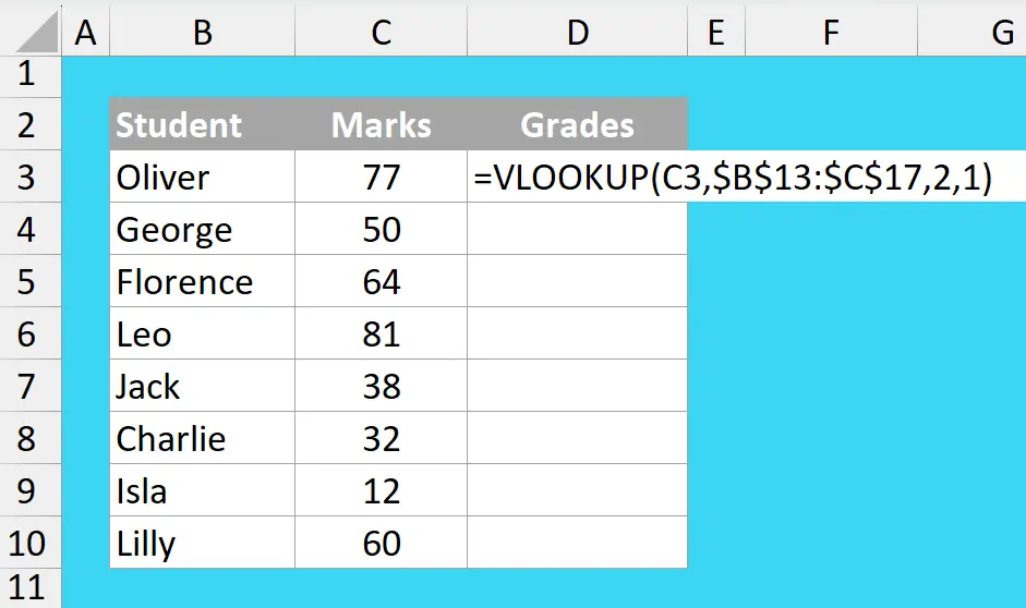
Remember to lock your table array with $ signs as given in this picture:
Conclusion:
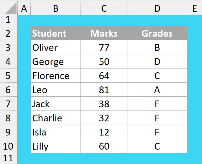
Here are the final grades perfect for each student. Remember the VLOOKUP approx will always search for the next lower value in the grading scheme as compared to the value being searched: