This tutorial will help you master the customization of any chart through a step by step guide.
The Dataset
These are the sales revenue by country. You can also use any other data set for your own business
The numbers were generated using RandBetween function, so that when the numbers update, you can see the animation ....

Here is the function applied to all cells in the ratings column
=Randbetween(5000,100000)
Your numbers will differ from mine as these are generated using RandBetween.
Steps involved
Step 1: In the next column create a formula to produce the highest value from the list.
For this we will use IF formula as follows:
=IF(C3>=MAX($C$3:$C$12),C3,0)
💡you will see that when we change anything in Excel sheet, the sales figures are re-generated and the new highest number is identified in the next column. This will help us in the bar chart.

These are the sales revenue by country. You can also use any other data set for your own business
The numbers were generated using RandBetween function, so that when the numbers update, you can see the animation of highest column ....
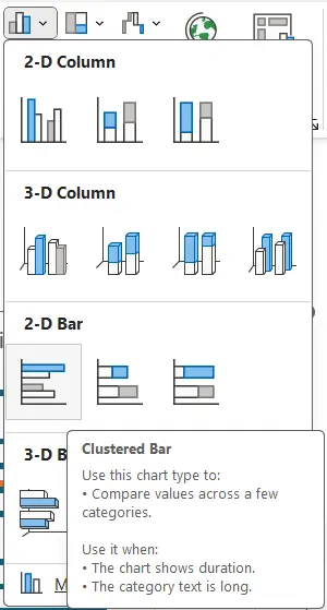
Step 2: Click anywhere in your table and insert a bar chart from the INSERT menu CHARTS group.
A default 2d bar chart will be inserted
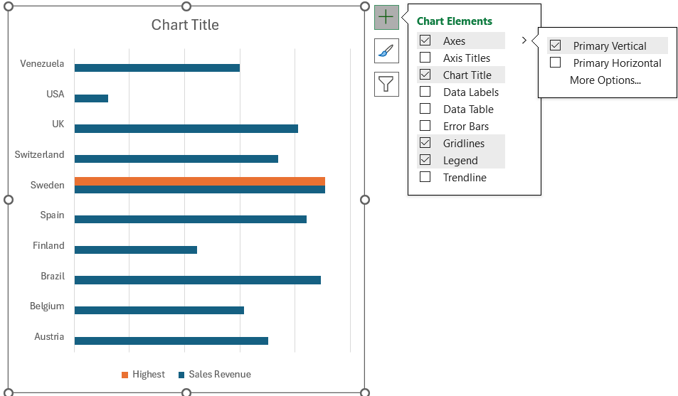
Step 3: Do some adjustments to make the chart look appealing like uncheck Gridlines and also Primary Horizontal Axis:
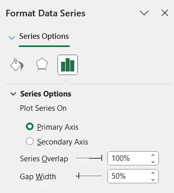
Step 4: Now click on any of the bars and in the chart menu Series Options on right of the screen do the following modifications:
- Make Series Overlap to 100%
- Adjust the Gap Width to 50%
Step 5: The final shape of the chart will be following where the highest bar is in front of the sales revenue bars, giving the effect that the bar is highlighted:
- Select the sales revenue bar and change its colour to grey
- Select the highest bar and change its colour to green
- Set the borders to dark

Step 6: The final chart will look like this:

Step 7: You have finally got it. Now refresh the data to see highest bar moving on.